
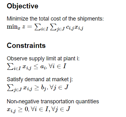
运输问题是一类特殊的线性规划问题,一般的运输问题就是要解决:把某种产品从若干个产地调运到若干个销地,在已知每个产地的供应量、每个销地的需求量、各地之间的运输单价的前提下,如何确定一个使得总的运输费用最小的方案。具体的数学模型和笔算求解可以参考中国大学MOOC上江西财经大学的运筹学课程。这个课程包含了运筹学要求掌握的所有问题,以及这些问题的单纯形法求解、excel求解,因此理论部分的介绍都可以参考这个课程,本文的实践主要基于pyomo和geatpy编程求解。
一、产销平衡的运输问题
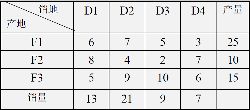
有三个工厂F1,F2,F3生产同种产品,它们的产量分别为25,15,10单位。该公司把这些产品分别运往四个销售点D1,D2,D3,D4 ,各销售点销量分别为13,21,9和7。从各工厂到各销售点的单位产品的运价为下表所示。问该公司应如何调运产品,在满足各销售点需求量的前提下,使总运费为最少
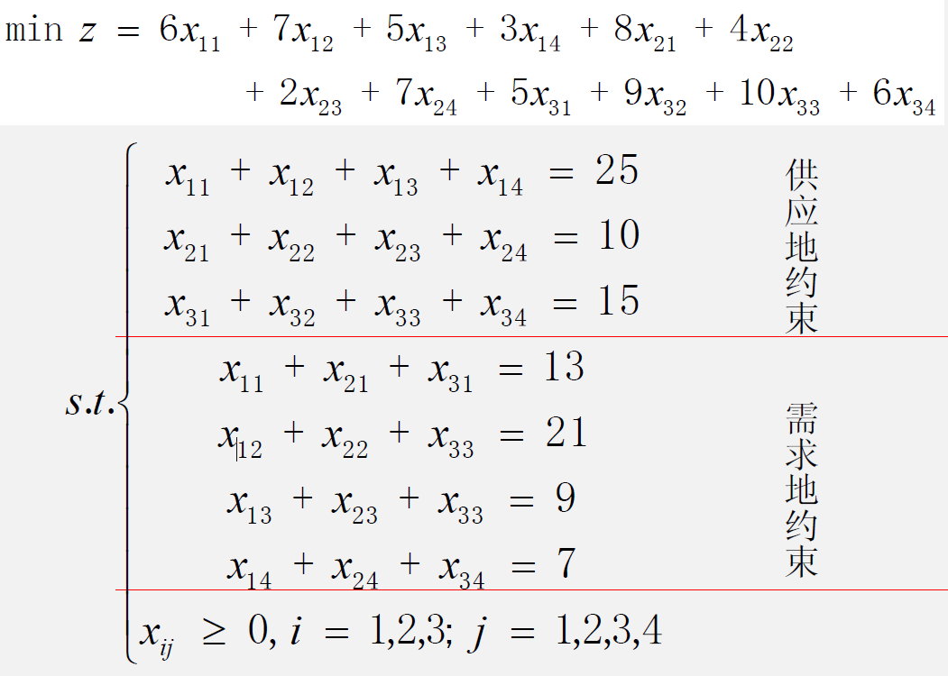
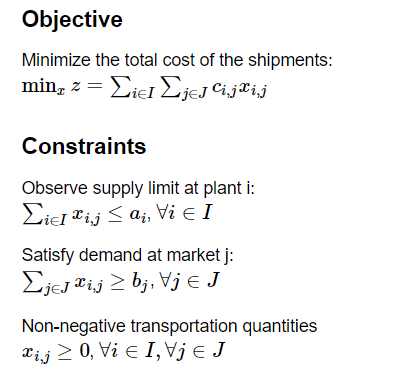
我们假设i产地(i属于{F1,F2,F3})运输到j销售地的数量为xij,则数学模型如下:
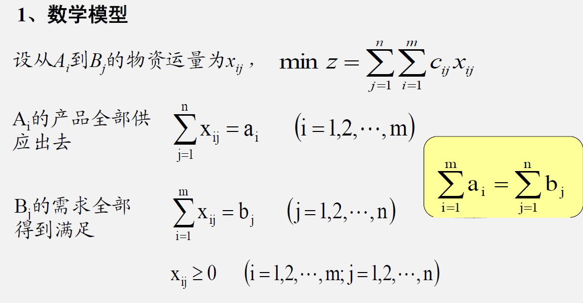
一般数学模型如下,其中cij是i到j的单位运价:
运输问题可以使用表上作业法进行人工求解,想要了解的可以看慕课,我们这里主要是讲述怎么利用编程工具pyomo和geatpy进行求解。
二、pyomo求解运输问题
1、数学模型
2、定义参数
首先定义好参数
# Import of the pyomo module
from pyomo.environ import *

# Creation of a Concrete Model
model = ConcreteModel()


# 定义生产地和销售地
## Define sets ##
#  Sets
#       i   canning plants   / seattle, san-diego /
#       j   markets          / new-york, chicago, topeka / ;
model.i = Set(initialize=['seattle','san-diego'], doc='Canning plans')
model.j = Set(initialize=['new-york','chicago', 'topeka'], doc='Markets')


# 定义生产地的生产量和销售地的需求量
## Define parameters ##
#   Parameters
#       a(i)  capacity of plant i in cases
#         /    seattle     350
#              san-diego   600  /
#       b(j)  demand at market j in cases
#         /    new-york    325
#              chicago     300
#              topeka      275  / ;
model.a = Param(model.i, initialize={'seattle':350,'san-diego':600}, doc='Capacity of plant i in cases')
model.b = Param(model.j, initialize={'new-york':325,'chicago':300,'topeka':275}, doc='Demand at market j in cases')


# 定义生产地到销售地的距离(千英里)
#  Table d(i,j)  distance in thousands of miles
#                    new-york       chicago      topeka
#      seattle          2.5           1.7          1.8
#      san-diego        2.5           1.8          1.4  ;
dtab = {
    ('seattle',  'new-york') : 2.5,
    ('seattle',  'chicago')  : 1.7,
    ('seattle',  'topeka')   : 1.8,
    ('san-diego','new-york') : 2.5,
    ('san-diego','chicago')  : 1.8,
    ('san-diego','topeka')   : 1.4,
    }
model.d = Param(model.i, model.j, initialize=dtab, doc='Distance in thousands of miles')


# 费用/千英里
#  Scalar f  freight in dollars per case per thousand miles  /90/ ;
model.f = Param(initialize=90, doc='Freight in dollars per case per thousand miles')


# cij就是产地i到销地j的单位运价
#  Parameter c(i,j)  transport cost in thousands of dollars per case ;
#            c(i,j) = f * d(i,j) / 1000 ;
def c_init(model, i, j):
 return model.f * model.d[i,j] / 1000
model.c = Param(model.i, model.j, initialize=c_init, doc='Transport cost in thousands of dollar per case')
3、定义变量
定义变量xij:
## Define variables ##
#  Variables
#       x(i,j)  shipment quantities in cases
#       z       total transportation costs in thousands of dollars ;
#  Positive Variable x ;
model.x = Var(model.i, model.j, bounds=(0.0,None), doc='Shipment quantities in case')
4、约束条件
## Define contrains ##
# supply(i)   observe supply limit at plant i
# supply(i) .. sum (j, x(i,j)) =l= a(i)
def supply_rule(model, i):
 return sum(model.x[i,j] for j in model.j) <= model.a[i]
model.supply = Constraint(model.i, rule=supply_rule, doc='Observe supply limit at plant i')
# demand(j)   satisfy demand at market j ;
# demand(j) .. sum(i, x(i,j)) =g= b(j);
def demand_rule(model, j):
 return sum(model.x[i,j] for i in model.i) >= model.b[j]
model.demand = Constraint(model.j, rule=demand_rule, doc='Satisfy demand at market j')
5、目标函数
## Define Objective and solve ##
#  cost        define objective function
#  cost ..        z  =e=  sum((i,j), c(i,j)*x(i,j)) ;
#  Model transport /all/ ;
#  Solve transport using lp minimizing z ;
def objective_rule(model):
 return sum(model.c[i,j]*model.x[i,j] for i in model.i for j in model.j)
model.objective = Objective(rule=objective_rule, sense=minimize, doc='Define objective function')
6、模型求解
展示模型结果:
## Display of the output ##
# Display x.l, x.m ;
def pyomo_postprocess(options=None, instance=None, results=None):
  model.x.display()
模型求解:
# This is an optional code path that allows the script to be run outside of
# pyomo command-line.  For example:  python transport.py
if __name__ == '__main__':
 # This emulates what the pyomo command-line tools does
 from pyomo.opt import SolverFactory
 import pyomo.environ
    opt = SolverFactory("glpk")
    results = opt.solve(model)
 #sends results to stdout
    results.write()
    print("\nDisplaying Solution\n" + '-'*60)
    pyomo_postprocess(None, model, results)
模型结果:
# ==========================================================
# = Solver Results                                         =
# ==========================================================
# ----------------------------------------------------------
#   Problem Information
# ----------------------------------------------------------
Problem:
- Name: unknown
  Lower bound: 153.675
  Upper bound: 153.675
  Number of objectives: 1
  Number of constraints: 6
  Number of variables: 7
  Number of nonzeros: 13
  Sense: minimize
# ----------------------------------------------------------
#   Solver Information
# ----------------------------------------------------------
Solver:
- Status: ok
  Termination condition: optimal
  Statistics:
    Branch and bound:
      Number of bounded subproblems: 0
      Number of created subproblems: 0
  Error rc: 0
  Time: 0.03862881660461426
# ----------------------------------------------------------
#   Solution Information
# ----------------------------------------------------------
Solution:
- number of solutions: 0
  number of solutions displayed: 0


Displaying Solution
------------------------------------------------------------
x : Shipment quantities in case
    Size=6, Index=x_index
    Key                       : Lower : Value : Upper : Fixed : Stale : Domain
     ('san-diego', 'chicago') :   0.0 :   0.0 :  None : False : False :  Reals
    ('san-diego', 'new-york') :   0.0 : 325.0 :  None : False : False :  Reals
      ('san-diego', 'topeka') :   0.0 : 275.0 :  None : False : False :  Reals
       ('seattle', 'chicago') :   0.0 : 300.0 :  None : False : False :  Reals
      ('seattle', 'new-york') :   0.0 :   0.0 :  None : False : False :  Reals
        ('seattle', 'topeka') :   0.0 :   0.0 :  None : False : False :  Reals
三、geatpy求解运输问题
1、定义参数
I = ['seattle','san-diego']
J = ['new-york','chicago', 'topeka']


# 定义生产地的生产量和销售地的需求量
a = {'seattle':350,'san-diego':600}
b = {'new-york':325,'chicago':300,'topeka':275}


# 定义生产地到销售地的距离(千英里)
#  Table d(i,j)  distance in thousands of miles
#                    new-york       chicago      topeka
#      seattle          2.5           1.7          1.8
#      san-diego        2.5           1.8          1.4  ;
dtab = {
    ('seattle',  'new-york') : 2.5,
    ('seattle',  'chicago')  : 1.7,
    ('seattle',  'topeka')   : 1.8,
    ('san-diego','new-york') : 2.5,
    ('san-diego','chicago')  : 1.8,
    ('san-diego','topeka')   : 1.4,
    }


# 费用/千英里
#  Scalar f  freight in dollars per case per thousand miles  /90/ ;
f = 90


# cij就是产地i到销地j的单位运价


def c_init(i, j):
 return f * dtab[i,j] / 1000


c = {}
for i in I:
 for j in J:
        c[i,j]=c_init(i,j)
2、约束条件
## Define contrains ##
# supply(i)   observe supply limit at plant i
# supply(i) .. sum (j, x(i,j)) =l= a(i)
def supply_rule(x, i):
 return sum(x[i,j] for j in J) - a[i]


# demand(j)   satisfy demand at market j ;
# demand(j) .. sum(i, x(i,j)) =g= b(j);
def demand_rule(x, j):
 return (-1)* sum(x[i,j] for i in I) + b[j]
3、目标函数
# 目标函数
def objective_rule(c,x):
 return sum(c[i,j]*x[i,j] for i in I for j in J)
4、建立模型
# -*- coding: utf-8 -*-
"""MyProblem.py"""
import numpy as np
import geatpy as ea


class MyProblem(ea.Problem): # 继承Problem父类
 def __init__(self):
        name = 'MyProblem' # 初始化name(函数名称,可以随意设置)
        M = 1 # 初始化M(目标维数)
        maxormins = [1]  # 初始化maxormins(目标最小最大化标记列表,1:最小化该目标;-1:最大化该目标)
        Dim = 6 # 初始化Dim(决策变量维数),这里就是产地*销地=2*3
        varTypes = [0] * Dim  # 初始化varTypes(决策变量的类型,元素为0表示对应的变量是连续的;1表示是离散的)
        lb = [0] * Dim  # 决策变量下界
        ub = [10000] * Dim  # 决策变量上界
        lbin = [1] * Dim  # 决策变量下边界(0表示不包含该变量的下边界,1表示包含),或者写作【1】*3
        ubin = [1] * Dim  # 决策变量上边界(0表示不包含该变量的上边界,1表示包含)
 # 调用父类构造方法完成实例化
        ea.Problem.__init__(self, name, M, maxormins, Dim, varTypes, lb, ub, lbin, ubin)


 def aimFunc(self, pop): # 目标函数
        Vars = pop.Phen  # 得到决策变量矩阵


        cnt = 0
        x = {}
        for i in I:
           for j in J:
                x[i, j] = Vars[:, [cnt]]
                cnt += 1


        pop.ObjV = objective_rule(c, x)  # 计算目标函数值,赋值给pop种群对象的ObjV属性,这里就是总运费


 # 采用可行性法则处理约束
 for i in I:
            pop.CV = np.hstack([
                supply_rule(x, i)  # i产地的总供应量小于他的总生产量
            ])


 for j in J:
            pop.CV = np.hstack([
                pop.CV, demand_rule(x, j)  # j销地的总供应量要大于他的总销售量,保证供应是充足的
            ])
5、模型求解
if __name__ == '__main__':
 """================================实例化问题对象==========================="""
    problem = MyProblem() # 生成问题对象
 """==================================种群设置==============================="""
    Encoding = 'RI' # 编码方式
    NIND = 100 # 种群规模
    Field = ea.crtfld(Encoding, problem.varTypes, problem.ranges, problem.borders) # 创建区域描述器
    population = ea.Population(Encoding, Field, NIND) # 实例化种群对象(此时种群还没被初始化,仅仅是完成种群对象的实例化)
 """================================算法参数设置============================="""
    myAlgorithm = ea.soea_DE_rand_1_L_templet(problem, population) # 实例化一个算法模板对象
    myAlgorithm.MAXGEN = 500 # 最大进化代数
    myAlgorithm.mutOper.F = 0.5 # 差分进化中的参数F
    myAlgorithm.recOper.XOVR = 0.7 # 重组概率
 """===========================调用算法模板进行种群进化======================="""
    [population, obj_trace, var_trace] = myAlgorithm.run() # 执行算法模板
    population.save() # 把最后一代种群的信息保存到文件中
 # 输出结果
    best_gen = np.argmin(problem.maxormins * obj_trace[:, 1]) # 记录最优种群个体是在哪一代
    best_ObjV = obj_trace[best_gen, 1]
    print('最优的目标函数值为:%s'%(best_ObjV))
    print('最优的决策变量值为:')
 for i in range(var_trace.shape[1]):
        print(var_trace[best_gen, i])
    print('有效进化代数:%s'%(obj_trace.shape[0]))
    print('最优的一代是第 %s 代'%(best_gen + 1))
    print('评价次数:%s'%(myAlgorithm.evalsNum))
    print('时间已过 %s 秒'%(myAlgorithm.passTime))
最终结果是,可以看出153.70会比pyomo求解的结果(153.675)差一下:
种群信息导出完毕。
最优的目标函数值为:153.7070860662967
最优的决策变量值为:
148.03609859240396
299.43385407422363
0.3649843431022787
176.9952992431655
0.5781097011820691
274.6734971806611
有效进化代数:500
最优的一代是第 492 代
评价次数:50600
时间已过 0.35503411293029785 秒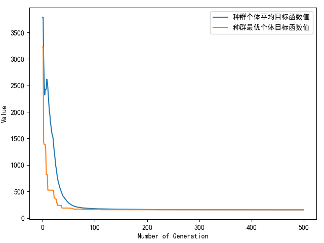
参考
【2】pyomo求解运输问题:https://nbviewer.jupyter.org/github/Pyomo/PyomoGallery/blob/master/transport/transport.ipynb