

当前的大语言模型已经拥有非常丰富的知识和技能,但很多能力仍然需要被进一步验证。其中最重要的一类能力,是能否从经验和教训中反思,并持续改进自己的 Skills。我们把这种能力称为后天学习 acquired learning。

Acquired learning refers to knowledge or skills gained through experience, education, or training.
在大语言模型系统里,这句话有一个很重要的工程含义:后天学习不一定要更新模型参数。预训练、后训练、强化学习、微调改变的是模型参数 theta;而 Skill、SOP、记忆、检索证据、失败案例、验证器反馈改变的是推理环境 C。
所以我们可以把 LLM Agent 的学习分成两条路:
参数训练学习:      theta -> theta'
非参数后天学习:    C_t -> C_{t+1}
Bayesian-Agent 做的是第二条路:不改 base model 的权重,而是从 verified trajectories 中学习 Skill 的可靠性、适用场景、失败模式和成本,让下一次推理拿到更好的条件。也就是经验和教训(成功的轨迹我们称之为经验,失败的轨迹我们称之为教训)。 也可以把它理解成一种归纳学习(inductive reasoning):先用演绎法搭建模型结构,再用归纳法,也就是贝叶斯更新,从数据中学习参数或假设。
系列文章更新中:
Bayesian Agent (一):让 Harness 与 Skills 的 Self-Evolving过程不再黑盒、没有方向,走向贝叶斯信念
Bayesian-Agent (二):不仅是又一个 agent framework,而是可跨 harness 的 Bayesian Evolution Layer
一、从三门问题开始:贝叶斯更新到底在更新什么
贝叶斯公式本身非常简单:
P(H | E) = P(E | H) P(H) / P(E)
其中:
| 符号 | 名称 | 含义 |
|---|---|---|
| H | Hypothesis / 假设 | 我们想判断真假的事情 |
| E | Evidence / 证据 | 我们观察到的新信息 |
| P(H) | Prior / 先验 | 看到证据之前,对假设的相信程度 |
| P(E | H) | Likelihood / 似然 | 如果假设为真,观察到该证据的概率 |
| P(H | E) | Posterior / 后验 | 看到证据之后,对假设的更新信念 |
| P(E) | Evidence / 边际概率 | 证据整体出现的概率,也起归一化作用 |
也可以写成更常用的比例形式:
posterior ∝ likelihood * prior
也就是:
新的信念 ∝ 证据在该假设下出现的概率 * 原来的信念
三门问题是最经典的贝叶斯直觉测试:
- 有三扇门,一扇门后面是车,另外两扇门后面是羊。
- 你先选一扇门,比如 A。
- 主持人知道答案,并打开另一扇有羊的门,比如 B。
- 你现在可以坚持 A,也可以换到 C。
很多人的直觉会说:现在只剩两扇门,所以 A 和 C 各有 1/2。但正确答案是:应该换门,换到 C 的胜率是 2/3。
关键点是:主持人的行为不是随机噪声,而是有条件的信息。主持人打开 B,不只是“少了一扇门”,而是在告诉你:“在知道车在哪的前提下,我选择打开了 B 这扇羊门。”
设:
H_A: 车在 A 后面
H_C: 车在 C 后面
O_B: 主持人打开 B
一开始:
P(H_A) = 1/3
P(H_B) = 1/3
P(H_C) = 1/3
当你选 A 后,主持人打开 B。因为主持人不会打开你选的门,也不会打开车门,所以:
P(O_B | H_A) = 1/2
P(O_B | H_C) = 1
P(O_B | H_B) = 0
用贝叶斯公式:
P(H_i | O_B) = P(O_B | H_i) P(H_i) / sum_j P(O_B | H_j) P(H_j)
这里的对应关系是:
| 项 | 三门问题里的含义 |
|---|---|
| Prior P(H_i) | 主持人开门前,车在每扇门后的概率 |
| Likelihood P(O_B | H_i) | 如果车在某扇门后,主持人打开 B 的概率 |
| Posterior P(H_i | O_B) | 主持人打开 B 后,车在某扇门后的概率 |
| Evidence P(O_B) | 主持人打开 B 这个事件整体发生的概率 |
于是:
P(H_A | O_B)
= (1/2 * 1/3) / (1/2 * 1/3 + 1 * 1/3 + 0 * 1/3)
= 1/3

P(H_C | O_B)
= (1 * 1/3) / (1/2 * 1/3 + 1 * 1/3 + 0 * 1/3)
= 2/3
flowchart LR
    A["Prior: 每扇门 1/3"] --> B["Observation: 主持人打开 B"]
    B --> C["Likelihood: P(O_B | H_i)"]
    C --> D["Posterior: A=1/3, C=2/3"]
    D --> E["Decision: 换门"]
严格说,三门问题讲的是贝叶斯更新。Agent 的运行轨迹更复杂:一次任务会同时产生 context、failure mode、token cost、tool turns、latency、metadata 等多个证据特征。Bayesian-Agent 需要的是一个能把这些特征转成 posterior belief 的 Bayesian Evidence Model。
二、Bayesian Evidence Model:当证据不止一个时怎么办
先看一个最小化的 categorical evidence model。给定一组特征 x,判断它属于哪个标签 y:
x = {x_1, x_2, ..., x_m}
y in {class_1, class_2, ...}
直接用贝叶斯公式:
P(y | x) = P(x | y) P(y) / P(x)
问题是 x 不是一个单独事件,而是一组特征:
P(y | x_1, x_2, ..., x_m)
= P(x_1, x_2, ..., x_m | y) P(y) / P(x_1, x_2, ..., x_m)
如果特征很多,直接估计联合概率 P(x_1, x_2, ..., x_m | y) 会非常困难。目前采用一个轻量的 factorized categorical likelihood:在给定标签 y 后,各个特征近似条件独立(即朴素贝叶斯的方案):
P(x_1, x_2, ..., x_m | y)
≈ Π_j P(x_j | y)
这里的 Π 是大写希腊字母 Pi,在数学里表示 product / 连乘。Π_j P(x_j | y) 的意思是:
P(x_1 | y) * P(x_2 | y) * ... * P(x_m | y)
于是:
P(y | x)
∝ P(y) Π_j P(x_j | y)
归一化以后得到:
P(y = c | x)
= P(c) Π_j P(x_j | c) / sum_{c'} P(c') Π_j P(x_j | c')
这里的对应关系是:
| 项 | Evidence model 里的含义 |
|---|---|
| Prior P(c) | 某个类别本来出现的概率 |
| Likelihood Π_j P(x_j | c) | 如果类别是 c,这些特征一起出现的概率近似 |
| Posterior P(c | x) | 看到这些特征后,样本属于类别 c 的概率 |
| Evidence P(x) | 这些特征整体出现的概率,通常用归一化分母处理 |
例子:一封邮件是不是垃圾邮件
假设我们要判断一封邮件是不是垃圾邮件:
y in {spam, normal}
观察到三个特征:
x_1 = contains_discount      # 邮件里出现“折扣”
x_2 = contains_link          # 邮件里有链接
x_3 = sender_unknown         # 发件人陌生
从历史邮件里统计到:
P(spam) = 0.30
P(normal) = 0.70

P(contains_discount | spam) = 0.80
P(contains_link | spam) = 0.70
P(sender_unknown | spam) = 0.60

P(contains_discount | normal) = 0.10
P(contains_link | normal) = 0.20
P(sender_unknown | normal) = 0.05
那么这封邮件是垃圾邮件的未归一化分数是:
score(spam)
= P(spam)
  * P(contains_discount | spam)
  * P(contains_link | spam)
  * P(sender_unknown | spam)

= 0.30 * 0.80 * 0.70 * 0.60
= 0.1008
普通邮件的未归一化分数是:
score(normal)
= P(normal)
  * P(contains_discount | normal)
  * P(contains_link | normal)
  * P(sender_unknown | normal)

= 0.70 * 0.10 * 0.20 * 0.05
= 0.0007
归一化:
P(spam | x)
= score(spam) / (score(spam) + score(normal))
= 0.1008 / (0.1008 + 0.0007)
≈ 0.993
所以模型会判断这封邮件大概率是垃圾邮件。
这个例子里:
| 概念 | 对应内容 |
|---|---|
| Prior | P(spam) 和 P(normal),历史上垃圾邮件/普通邮件的比例 |
| Likelihood | P(contains_discount | spam) 等特征在某类邮件下出现的概率 |
| Posterior | P(spam | x),看到这些特征后邮件是垃圾邮件的概率 |
| Factorization assumption | 给定 spam 或 normal 后,折扣、链接、陌生发件人近似独立 |
这就是 categorical evidence model 的直觉:它不需要理解“折扣”和“链接”的深层语义,只要不断从历史样本里统计“哪些特征经常和哪个标签一起出现”,就可以做出可解释的概率判断。在 Bayesian-Agent 里,它被定位为第一个可解释 evidence backend,而不是方法的上限。
三、人的后天学习:一个技能是如何从经验里长出来的
假设一个人正在学习写 SQL 报表。他不是从零拥有“SQL 专家能力”的。最开始,他可能已经知道一些语法:
SELECT, WHERE, GROUP BY, HAVING, ORDER BY
这相当于他的先验知识。可是,真正做任务时,他会不断遇到经验和教训:
- 有些任务需要先读表结构,否则会写错列名。
- 有些任务需要
GROUP BY,否则聚合结果错误。 - 有些任务要求“只输出一条 SQL”,如果写解释文字就会失败。
- 有些更新任务不能带自增主键列。
- 有些失败不是知识不会,而是没有验证输出。
每一次任务之后,如果有老师、测试用例或数据库执行结果给出反馈,那么这个人就会获得一条 evidence:
e_i = (x_i, y_i)
其中:
x_i = {
  task_type,
  schema_complexity,
  required_operator,
  failure_mode,
  verification_signal
}

y_i in {success, failure}
如果我们把“先读 schema、再写 SQL、最后执行验证”看成一条 Skill hypothesis h_sql_verify,为了避免记号太长,可以把“在这条 Skill 作用域下的概率”写成 P_h(...),其中:
h = h_sql_verify
P_h(y | x) 等价于 P(y | x, h_sql_verify)
这和前面垃圾邮件例子里的 P(spam | x) 是同一种结构。垃圾邮件例子里,分类器或历史邮件统计这个“模型作用域”是隐含的;到了 Skill 学习里,我们把它显式写出来,因为不同 Skill 会有不同的历史证据和成功率。
于是后天学习可以写成:
P_h(success | x)
∝ P_h(success) Π_j P_h(x_j | success)
更完整地写,就是:
P_h(y | x)
= P_h(y) Π_j P_h(x_j | y)
  / sum_{y'} P_h(y') Π_j P_h(x_j | y')
这里的 prior、likelihood、posterior 可以一一对应:
| 贝叶斯概念 | 后天学习里的含义 |
|---|---|
| Prior P_h(y) | 在这条 Skill 作用域下,看到当前任务特征前的历史成功/失败倾向 |
| Likelihood Π_j P_h(x_j | y) | 如果这次会成功或失败,那么当前这些任务特征出现的概率 |
| Posterior P_h(y | x) | 看到当前任务特征后,这条 Skill 成功或失败的更新概率 |
| Evidence P_h(x) | 在这条 Skill 作用域下,当前任务特征整体出现的概率,用分母归一化 |
举一个很小的数值例子。学习者过去用 h_sql_verify 做过 10 个 SQL 任务,其中 6 次成功、4 次失败。用 alpha = 1 做平滑:
P_h(success) = (6 + 1) / (10 + 2) = 7/12
P_h(failure) = (4 + 1) / (10 + 2) = 5/12
这就是 prior。现在来了一个新任务,它的特征是:
x_1 = task_type=aggregation
x_2 = required_operator=GROUP_BY
x_3 = verification_signal=executed_ok
从过去经验里统计到:
P_h(task_type=aggregation | success) = 4/6
P_h(required_operator=GROUP_BY | success) = 4/6
P_h(verification_signal=executed_ok | success) = 5/6

P_h(task_type=aggregation | failure) = 3/4
P_h(required_operator=GROUP_BY | failure) = 1/4
P_h(verification_signal=executed_ok | failure) = 1/4
这些就是 likelihood。于是:
score(success)
= 7/12 * 4/6 * 4/6 * 5/6
≈ 0.216

score(failure)
= 5/12 * 3/4 * 1/4 * 1/4
≈ 0.0195

P_h(success | x)
= 0.216 / (0.216 + 0.0195)
≈ 0.917
这就是 posterior。人的直觉说法是:“这类任务我已经掌握了,只要按 checklist 执行验证,成功率很高。”贝叶斯说法是:“在这条 Skill 和这些 evidence features 下,posterior success probability 升高了。”
如果一个学习者反复观察到:
task_type = aggregation
required_operator = GROUP BY
verification_signal = executed_ok
这些特征经常和成功一起出现,那么这条 Skill 的 posterior success 就会上升。相反,如果:
failure_mode = missing_group_by
verification_signal = not_executed
经常和失败一起出现,那么学习者会形成一个新的经验:
遇到聚合任务时,不要只写 SELECT;必须检查 GROUP BY/HAVING,并执行验证。
这就是后天学习。人的大脑参数当然也会变化,但从工程视角看,很多可复用的能力沉淀在外部结构里:
- 笔记
- checklist
- SOP
- 失败案例本
- 测试习惯
- 反思模板
- 面向场景的操作策略
在 LLM Agent 里,这些外部结构就是 Skills、SOPs、memory、tool traces 和 verifier feedback。它们不改变 theta,但改变下一次推理的条件:
P(X | theta) -> P(X | theta, C)
更进一步,后天学习就是让 C 随经验更新:
C_{t+1} = Update(C_t, evidence_t)
flowchart TD
    A["Task"] --> B["Attempt with current Skill"]
    B --> C["Verifier / Teacher Feedback"]
    C --> D["Evidence: context, outcome, failure mode"]
    D --> E["Belief update"]
    E --> F["Skill patch / split / compress / retire"]
    F --> G["Better Skill context for next task"]
    G --> A
这和参数训练不同。参数训练是在改变模型内部的 theta。后天学习是在改变模型外部的 C,让同一个模型在下一次推理时拥有更好的证据、更好的步骤、更好的失败规避策略。
四、Bayesian-Agent:把 Skill 当成可验证的假设
Bayesian-Agent 的核心观点是:
Skill/SOP 不是一段神圣的提示词,而是一个关于“如何让 Agent 成功”的 hypothesis。
记:
h_k = 第 k 条 Skill/SOP hypothesis
x = 当前任务和运行证据特征
y in {success, failure}
大语言模型本身拥有丰富知识:
P(X | theta)
Agent 系统则会把模型放进某个推理环境里:
P(X | theta, C)
这里的 C 包括 prompt、tools、memory、RAG、Skill、SOP、历史轨迹和 verifier feedback。Bayesian-Agent 不直接更新 theta,而是更新 C 中的 Skill belief:
P_{h_k}(success | x)
这里的 P_{h_k}(...) 表示“在第 k 条 Skill/SOP 的证据作用域下计算概率”。它等价于 P(success | x, h_k),只是把 h_k 放到下标里,避免读者把 h_k 误解成和 x 同级的普通特征。
每次 Agent 跑完一个任务,Bayesian-Agent 会收集一条 verified trajectory:
e_i = {
  task_id,
  skill_id,
  context,
  outcome,
  failure_mode,
  input_tokens,
  output_tokens,
  total_tokens,
  turns,
  elapsed_seconds,
  metadata
}
这些 evidence 进入 Skill registry,形成每条 Skill 的 posterior belief。
在 Bayesian-Agent 里,对应关系是:
| 贝叶斯概念 | Bayesian-Agent 里的含义 |
|---|---|
| Hypothesis h_k | 第 k 条 Skill/SOP |
| Evidence e_i | 一次经过验证的 agent trajectory |
| Feature x_i | context、failure_mode、token_bucket、turn_bucket、latency_bucket、metadata |
| Label y_i | verified outcome: success 或 failure |
| Prior P_{h_k}(y) | 这条 Skill 在已有轨迹里的平滑成功/失败基率 |
| Likelihood P_{h_k}(x_j | y) | 某个 evidence feature 在成功/失败轨迹中出现的概率 |
| Posterior P_{h_k}(y | x) | 给定当前任务特征后,这条 Skill 成功/失败的更新概率 |
五、Benchmark 例子:从零进化、失败改写与增量修复
上面的公式还是抽象。下面看几组 benchmark 轨迹,分别展示三种情况:
clean full mode:  从零开始跑,但一路成功,只展示 reliability posterior 上升
failure-in-loop:  从零开始跑,中途失败,posterior failure 上升并触发 Skill rewrite
incremental mode: 读取 baseline 失败,posterior 记录 failure mode,再只重跑失败任务
例子 A:从零 clean run 时,posterior 如何持续升高
在 full mode 里,Bayesian-Agent 不读取 GA baseline 失败轨迹,而是从空 registry 开始:
success = 0
failure = 0
P_h(success) = 1 / 2 = 0.500
rewrite = explore
每完成一个任务,benchmark verifier 会给出 success 或 failure。Bayesian-Agent 立刻把这条 trajectory 写入 Skill registry,然后下一道题拿到更新后的 posterior-weighted Skill context。
这和“最后统一总结一次经验”不同。它是在线更新:
task_i -> verifier -> evidence_i -> registry_i+1 -> context_i+1 -> task_i+1
SOP-Bench full mode
SOP-Bench 从零跑时,前几个任务逐步覆盖了不同决策类型:
| Task | Expected/Got | Verified outcome | 更新后的 P_h(success) | Rewrite action |
|---|---|---|---|---|
| before sop_01 | no evidence | - | 0.500 | explore |
| sop_01 | fulfill_immediately | success | 0.667 | explore |
| sop_02 | fulfill_immediately | success | 0.750 | explore |
| sop_03 | fulfill_delayed | success | 0.800 | compress |
| sop_04 | backorder | success | 0.833 | compress |
| sop_05 | reject | success | 0.857 | compress |
| after 10 tasks | mixed SOP decisions | 10⁄10 success | 0.917 | compress |
| after 20 tasks | all SOP tasks | 20⁄20 success | 0.955 | compress |
这些数值来自 Laplace smoothing:
P_h(success) = (success + 1) / (success + failure + 2)
例如,完成 5 个 SOP 任务且全部成功后:
P_h(success) = (5 + 1) / (5 + 0 + 2) = 6/7 ≈ 0.857
这里 Skill 的“持续改写”不是每一步都让 LLM 重新写一份长 SOP,而是让 Skill context 持续被 posterior 校准:
0 条证据: 先探索,遵循基础 guardrails
1-2 条成功证据: posterior 上升,但仍保持 explore
3 条以上稳定成功: rewrite action 变成 compress,说明这条 Skill 已经稳定
持续成功: context 继续保留更高 posterior 和更低不确定性
也就是说,从零跑时,Bayesian-Agent 学到的是:
这条 SOP-Bench Skill 在当前 harness/model/context 下越来越可靠。
最终 full mode 结果:
SOP-Bench full mode: 20/20 = 100%
posterior_success: 0.955
Lifelong AgentBench full mode
Lifelong AgentBench 从零跑时,也同样在线更新。前几个任务覆盖了 INSERT、SELECT、UPDATE、GROUP BY/HAVING 等 SQL 技能:
| Task | SQL pattern | Verified outcome | 更新后的 P_h(success) | Rewrite action |
|---|---|---|---|---|
| before lifelong_0 | no evidence | - | 0.500 | explore |
| lifelong_0 | INSERT without extra id column | success | 0.667 | explore |
| lifelong_1 | SELECT with filter/limit | success | 0.750 | explore |
| lifelong_2 | GROUP BY + ORDER BY | success | 0.800 | compress |
| lifelong_3 | UPDATE mutation | success | 0.833 | compress |
| lifelong_4 | GROUP BY + HAVING | success | 0.857 | compress |
| after 10 tasks | mixed SQL tasks | 10⁄10 success | 0.917 | compress |
| after 20 tasks | all Lifelong tasks | 20⁄20 success | 0.955 | compress |
最终 full mode 结果:
Lifelong AgentBench full mode: 20/20 = 100%
posterior_success: 0.955
这个 clean run 展示的是“正向经验”的后天学习:每个 verified success 都会提高这条 Skill 在当前 context 下的 posterior reliability。
要说明“失败 -> 改写 Skill -> 后面类似 case 做对”这条链路,还需要一条带失败的在线轨迹。
例子 B:从零跑,中途失败如何触发 Skill rewrite
以 SOP-Bench 的 CSV 写回错误为例。这条轨迹展示同一套 Bayesian update 在“从空 registry 开始,但中途遇到失败”时的行为。
初始时只有一条基础 Skill:
h_base = benchmark/sop_bench
success = 0
failure = 0
P_h_base(success) = 0.500
rewrite = explore
前两题成功:
sop_01: success
sop_02: success

P_h_base(success)
= (2 + 1) / (2 + 0 + 2)
= 0.750
这时系统还不会改写 Skill,只会认为基础 SOP skill 在当前 harness 下初步可靠。
接下来出现两个相似失败:
sop_13: failure, failure_mode = left_expected_output_blank
sop_14: failure, failure_mode = left_expected_output_blank
也就是 Agent 算出了流程,却没有把目标 CSV 行的 expected_output 写成非空值。当前观测到的任务特征是:
context = sop_bench
metadata.output_contract = csv_expected_output
failure_mode = left_expected_output_blank
这里的 failure_mode = left_expected_output_blank 表示“expected_output 留空”这个具体错误类型;它不是 failure 标签本身。
此时基础 Skill 的证据是:
success = 2
failure = 2
所以 class prior 是:
P_h_base(success) = (2 + 1) / (4 + 2) = 0.500
P_h_base(failure) = (2 + 1) / (4 + 2) = 0.500
再看关键 feature 的 likelihood。failure_mode 是这次失败中最关键的特征;真实实现还会把 context、token bucket、turn bucket、latency bucket 和 metadata 一起连乘进去。
在两条成功轨迹里,failure_mode = left_expected_output_blank 出现了 0 次;在两条失败轨迹里,它出现了 2 次。用 Laplace smoothing:
P_h_base(failure_mode = left_expected_output_blank | success)
= (0 + 1) / (2 + 2)
= 0.250

P_h_base(failure_mode = left_expected_output_blank | failure)
= (2 + 1) / (2 + 2)
= 0.750
于是 Bayesian Evidence Model 的 posterior 如下:
score_success
= P(success) * P(failure_mode = left_expected_output_blank | success)
= 0.500 * 0.250
= 0.125

score_failure
= P(failure) * P(failure_mode = left_expected_output_blank | failure)
= 0.500 * 0.750
= 0.375

P_h_base(
    failure
  | context = sop_bench,
    metadata.output_contract = csv_expected_output,
    failure_mode = left_expected_output_blank
)
= 0.375 / (0.125 + 0.375)
= 0.750

P_h_base(
    success
  | context = sop_bench,
    metadata.output_contract = csv_expected_output,
    failure_mode = left_expected_output_blank
)
= 0.250
这一步很重要:失败不是让系统“更相信原来的 Skill”,而是让系统更相信:
在 context = sop_bench, metadata.output_contract = csv_expected_output,
failure_mode = left_expected_output_blank 这个条件下,
h_base 很可能继续失败。
因此 rewrite policy 不应该 compress,而应该 patch 或 split:
rewrite = patch
reason = failures cluster around left_expected_output_blank
改写后的 Skill context 不是泛泛地说“仔细一点”,而是把失败模式变成可执行约束。当前实现会在下一轮 prompt 里注入类似这样的 patch section:
### Bayesian Failure-Mode Patches: sop_bench
- failure_mode=left_expected_output_blank observed=2
  - After writing, re-read test_set_with_outputs.csv and confirm the target row's expected_output is non-empty.
  - If the target cell is empty, write the computed raw category string before finishing.
然后用改写后的 Skill context 继续处理相似任务。后续成功会回写到同一条 benchmark Skill;失败历史不会被洗掉,posterior 会在保留 failure-mode 记忆的同时重新上升:
| Step | Evidence | Prior | Likelihood signal | Posterior | Skill action |
|---|---|---|---|---|---|
| before rewrite | 2 success + 2 failure | P_h_base(success)=0.500 | recurring empty output failure | 0.500 | patch |
| retry sop_13 | repaired success | 0.500 | patch applied and verified | (3+1)/(5+2)=0.571 | keep patch |
| retry sop_14 | similar repaired success | 0.571 | same CSV writeback contract | (4+1)/(6+2)=0.625 | keep patch |
| later sop_20 | similar output-contract case succeeds | 0.625 | left_expected_output_blank no longer appears | (5+1)/(7+2)=0.667 | less uncertain |
这就是“持续改写 Skill -> 后验持续升高”的完整链条:
先验:
  h_base 对 SOP-Bench 只有不确定的成功率

失败证据:
  expected_output 留空这个失败模式连续出现

似然:
  P(failure_mode = left_expected_output_blank | failure)
  远高于
  P(failure_mode = left_expected_output_blank | success)

后验:
  P_h_base(failure | context=sop_bench, metadata.output_contract=csv_expected_output,
  failure_mode=left_expected_output_blank) 上升到 0.750

rewrite:
  注入 failure-mode-specific patch context,显式约束 raw category + non-empty verification

后续相似 case:
  带 patch context 的 Skill 连续成功

新的后验:
  P_h_base(success) 从 0.500 -> 0.571 -> 0.625 -> 0.667
换句话说,Bayesian-Agent 里的“后验升高”有两种不同含义:
正向经验:
  success evidence 让同一条 Skill 的 posterior_success 升高

失败改写:
  failure evidence 先让原 Skill 在某个条件下的 posterior_failure 升高,
  触发 patch/split,
  然后带 patch context 的后续成功轨迹把 posterior_success 拉高
例子 C:SOP-Bench 写错 CSV 输出格式
SOP-Bench 的任务要求 Agent 阅读 sop.txt、tools.py 和目标 CSV 行,然后把原始决策字符串写回 expected_output 单元格。例如:
manual_review
backorder
fulfill_immediately
GA baseline 在 deepseek-v4-flash 上的 SOP-Bench 结果是:
16 / 20 = 80%
其中一个失败任务是 sop_12:
| 项 | 内容 |
|---|---|
| Expected | manual_review |
| Baseline got | <final_decision>manual_review</final_decision> |
| Failure mode | wrote_xml_tags_in_csv_expected_output |
| 失败原因 | 语义对了,但写入 CSV 的格式错了;benchmark 只接受 raw category string |
还有三个失败任务 sop_13、sop_14、sop_20 的共同问题是:
| 项 | 内容 |
|---|---|
| Expected | backorder 或 fulfill_immediately |
| Baseline got | 空字符串 |
| Failure mode | left_expected_output_blank |
| 失败原因 | 没有把目标行的 expected_output 写成非空值,或者没有验证写回结果 |
这些失败会进入 Bayesian-Agent 的 evidence:
e_i = {
  skill_id: benchmark/sop_bench,
  context: sop_bench,
  outcome: failure,
  failure_mode: wrote_xml_tags_in_csv_expected_output 或 left_expected_output_blank,
  token_bucket: 10k_100k,
  ...
}
在 baseline 之后,benchmark/sop_bench 这条 Skill 的标签统计是:
success = 16
failure = 4
用 alpha = 1 平滑:
P_h(success) = (16 + 1) / (20 + 2) ≈ 0.773
P_h(failure) = (4 + 1) / (20 + 2) ≈ 0.227
更重要的是,failure mode 的似然被记录下来:
P_h(failure_mode=left_expected_output_blank | failure) 较高
P_h(failure_mode=wrote_xml_tags_in_csv_expected_output | failure) 被显式记录
于是下一次 Bayesian context 不是泛泛地说“做得更好”,而是把失败转成更具体的 SOP guardrails:
- Read sop.txt, tools.py, and the target CSV row before acting.
- The requested row is one-indexed after the header; update rows[row_index - 1].
- Compute only the target row and write only its expected_output cell.
- Write the raw category string only; never write XML tags, Markdown, quotes, or explanations.
- Verify the target row's expected_output is non-empty before finishing.
这就是 Skill 的后天学习:失败不是被丢掉,而是变成下一次推理环境里的条件。
incremental repair 只重跑 4 个失败任务,结果是:
| Task | Baseline | Bayesian repair |
|---|---|---|
| sop_12 | <final_decision>manual_review</final_decision> | manual_review |
| sop_13 | 空字符串 | backorder |
| sop_14 | 空字符串 | fulfill_immediately |
| sop_20 | 空字符串 | fulfill_immediately |
最终:
SOP-Bench: 16/20 -> 20/20
Accuracy: 80% -> 100%
Repair cost: 256k extra tokens
注意,这里 Bayesian-Agent 没有把失败样本从记忆中删除。修复成功后,registry 里仍然保留 4 条失败 evidence 和 4 条 repair success evidence:
success = 20
failure = 4
P_h(success) = (20 + 1) / (24 + 2) ≈ 0.808
这很重要:posterior belief 不是盲目乐观地变成 100%,而是保留“这条 Skill 曾经在这些 failure modes 上出错”的校准信息。最终任务成功率变成 100%,是因为失败任务被带着更好的 Skill context 重跑并修好了。
例子 D:Lifelong-Bench SQL 任务写入了不该写的列
Lifelong AgentBench 的任务要求 Agent 根据 task.json 生成 SQL,并用数据库执行结果验证。
GA baseline 在 deepseek-v4-flash 上的 Lifelong 结果是:
18 / 20 = 90%
其中一个失败任务是 lifelong_0。任务要求插入会员支付记录,正确 SQL 是:
INSERT INTO membership_payments
  (member_id, payment_date, amount, payment_method)
VALUES
  (102, '2023-10-15', 75, 'Credit Card');
baseline 写成了:
INSERT INTO membership_payments
  (payment_id, member_id, payment_date, amount, payment_method)
VALUES
  (26, 102, '2023-10-15', 75, 'Credit Card');
它多写了 payment_id,也就是自增主键/未请求列。Bayesian-Agent 将其归入:
failure_mode = invented_unrequested_column
另一个失败任务是 lifelong_19。baseline 没有只写 SQL,而是把 agent transcript 也写进了答案,导致执行时报错:
near "Turn": syntax error
Bayesian-Agent 将其归入:
failure_mode = wrote_transcript_instead_of_sql_after_workspace_confusion
这两类失败进入 registry:
success = 18
failure = 2

P_h(success) = (18 + 1) / (20 + 2) ≈ 0.864
P_h(failure) = (2 + 1) / (20 + 2) ≈ 0.136
下一次 Lifelong context 会突出这些教训:
- Read task.json in the current workspace; do not inspect sibling benchmark runs.
- Write exactly one SQL statement to answer.sql; no Markdown and no explanation.
- Use only columns present in task.json unless the instruction explicitly asks for a new value.
- For INSERT statements, do not include id or primary-key columns unless the instruction explicitly provides their values.
- For mutation tasks, write executable SQL that reproduces the expected table state.
repair 只重跑两个失败任务:
| Task | Baseline failure | Bayesian repair |
|---|---|---|
| lifelong_0 | 多写 payment_id | 去掉 payment_id,只插入指定字段 |
| lifelong_19 | 把 transcript 写进 SQL | 只输出一个可执行 DELETE SQL |
最终:
Lifelong AgentBench: 18/20 -> 20/20
Accuracy: 90% -> 100%
Repair cost: 122k extra tokens
这几组例子说明:Bayesian-Agent 的“持续改进 Skill”不是一句口号,而是三条可检查的链条。
从零 clean run 时:
成功轨迹
-> Bayesian Evidence Model posterior 上升
-> rewrite action 从 explore 变成 compress
-> posterior-weighted Skill context 更稳定
-> 下一轮任务继续验证
从零 failure-in-loop 时:
失败轨迹
-> failure feature 的 likelihood 被记录
-> 原 Skill 在相似条件下的 posterior_failure 上升
-> rewrite action 变成 patch 或 split
-> rewritten Skill 处理相似 case
-> 成功轨迹回写 registry
-> rewritten Skill 的 posterior_success 上升
增量修复时:
失败轨迹
-> failure_mode
-> Bayesian Evidence Model belief update
-> posterior-weighted Skill context
-> 只重跑失败任务
-> 成功轨迹回写 registry
-> 下一轮 Skill 更可靠
六、从 Beta-Bernoulli 到 Bayesian Evidence Model
最简单的贝叶斯 Skill update 是 Beta-Bernoulli。对一条 Skill h_k,只看成功和失败次数:
p_k ~ Beta(alpha_0, beta_0)
y_i ~ Bernoulli(p_k)
观察到 s_k 次成功、f_k 次失败后:
p_k | D_k ~ Beta(alpha_0 + s_k, beta_0 + f_k)
E[p_k | D_k] = (alpha_0 + s_k) / (alpha_0 + beta_0 + s_k + f_k)
这个模型很清晰,但它有一个问题:它只知道“这条 Skill 总体成功率是多少”,不知道“它在哪类 context 下成功,在哪类 failure mode 下失败”。
于是我们升级到 feature-conditioned Bayesian Evidence Model。
Bayesian-Agent 当前默认把每条 Skill 的 evidence 特征离散化:
x = {
  context,
  failure_mode,
  token_bucket,
  turn_bucket,
  latency_bucket,
  metadata.*
}
对每条 Skill h_k,维护:
P_{h_k}(y) = (N_y + alpha) / (N + alpha * |Y|)

P_{h_k}(x_j = v | y)
= (N_{j,v,y} + alpha) / (N_{j,y} + alpha * |V_j|)
预测当前 context 下这条 Skill 的成功率:
P_{h_k}(y = success | x)
∝ P_{h_k}(y = success) Π_j P_{h_k}(x_j | y = success)
完整归一化形式是:
P_{h_k}(y = success | x)
= score(success) / (score(success) + score(failure))

score(y)
= P_{h_k}(y) Π_j P_{h_k}(x_j | y)
其中:
-
N_y是这条 Skill 下某个标签的次数。 -
N_{j,v,y}是在标签y下,第j个特征取值为v的次数。 -
|V_j|是第j个特征的取值空间大小。 -
alpha = 1是 Laplace smoothing,用来避免未见过的特征导致概率为 0。
直觉上,这相当于让 Agent 形成这样的经验:
这条 Skill 在 SOP-Bench 上通常成功。
这条 Skill 遇到 missing_group_by 这类 failure mode 时要 patch。
这条 Skill 在高 token bucket 下可能变慢。
这条 Skill 在 SQL mutation tasks 里必须先检查主键列。
它不是凭感觉记忆,而是把每次 verified outcome 变成条件概率。
七、Bayesian-Agent 的后天学习闭环
Bayesian-Agent 的 acquired learning loop 可以写成:
S_t = Skill registry at time t
e_t = verified trajectory evidence
S_{t+1} = BayesianUpdate(S_t, e_t)
C_{t+1} = RenderContext(S_{t+1}, task_context)
下一次推理变成:
P(X | theta, C_{t+1})
也就是说,模型参数没变,但推理条件变了。Agent 不再只是“带着一长串记忆继续猜”,而是拿到 posterior-weighted Skill context:
Use these Skills/SOPs as hypotheses, not as unquestioned instructions.
- skill_a: algorithm=categorical_bayes, posterior_success=0.95, context_success=0.92, rewrite=compress
- skill_b: algorithm=categorical_bayes, posterior_success=0.42, context_success=0.21, rewrite=patch
flowchart LR
    A["Base LLM: theta fixed"] --> B["Agent Harness"]
    B --> C["Task Execution"]
    C --> D["Verifier"]
    D --> E["Trajectory Evidence"]
    E --> F["Bayesian Evidence Registry"]
    F --> G["Posterior-weighted Skill Context"]
    G --> B
这个过程有三个重要特征:
- 从零学习:没有历史 traces 时,Agent 也可以边跑任务边积累 evidence。
- 增量修复:已有 Agent 跑失败的任务,可以只把失败轨迹交给 Bayesian-Agent,然后只重跑失败项。
- 跨 harness 适配:只要外部 Agent 能产出 trajectory evidence,并能接收 Skill context,就可以接入。
八、为什么这是 LLM Agent 的关键能力
当前的大语言模型知识和技能已经非常丰富。很多时候,模型不是“不知道”,而是:
- 没有检查当前文件。
- 没有验证工具输出。
- 没有识别失败模式。
- 没有把上次失败转化成下一次的约束。
- 没有区分这个 Skill 在哪个 context 下可靠。
这就是为什么后天学习很重要。Agent 不应该只依赖参数里的通用能力,也应该有一套运行时的学习机制:
experience -> evidence -> posterior belief -> better Skill -> better context -> better run
在我们的 deepseek-v4-flash 实验里,新的 Bayesian Evidence Model backend 已经可以作为 acquired learning layer 工作:
| Benchmark | Agent | Accuracy | Input Tokens | Output Tokens | Total Tokens | Efficiency |
|---|---|---|---|---|---|---|
| SOP-Bench | GA baseline | 80% | 1.34M | 57k | 1.39M | 11.47 |
| SOP-Bench | Bayesian Evidence full | 100% | 1.13M | 57k | 1.19M | 16.82 |
| SOP-Bench | Bayesian Evidence incremental | 100% | 245k extra | 12k extra | 256k extra | 15.60 |
| Lifelong AgentBench | GA baseline | 90% | 649k | 42k | 690k | 26.07 |
| Lifelong AgentBench | Bayesian Evidence full | 100% | 660k | 48k | 708k | 28.26 |
| Lifelong AgentBench | Bayesian Evidence incremental | 100% | 112k extra | 9k extra | 122k extra | 16.40 |
这组结果说明两件事。
第一,从零运行时,Bayesian-Agent 可以把 verified trajectories 变成 Skill evidence,并在后续任务中持续利用这些 evidence。
第二,增量模式更接近生产环境:一个已有 Agent 先跑,Bayesian-Agent 读取失败轨迹,只对失败任务进行 posterior-guided repair。它不是替换原来的 Agent,而是成为一个即插即用的后天学习层。
九、一个更准确的定义
我们可以把 Bayesian-Agent 的 acquired learning 定义为:
Acquired learning for agents is the non-parametric improvement of task behavior
by updating external Skill/SOP beliefs from verified experience,
without changing the base model parameters.
也就是说:
Agent 的后天学习,是指在不更新 base model 参数的情况下,
通过验证过的经验和教训,更新外部 Skill/SOP belief,
从而改善后续任务行为的非参数学习过程。
这里的“非参数”不是说整个系统没有参数,而是说它不更新 LLM 的权重 theta。它更新的是外部推理环境:
theta 固定
C 持续进化
Skill belief 持续被 evidence 校准
这也是 Bayesian-Agent 想表达的核心范式:
Pre-training gives the model knowledge.
Post-training aligns the model behavior.
Acquired learning lets the agent learn from its own verified experience.
预训练给模型知识,后训练塑造模型行为,后天学习让 Agent 从自己的经验和教训里持续进化。
十、为什么需要贝叶斯???
有人会说,其实目前方法的本质也还是根据执行轨迹,看错哪里了去针对性的改skill, 那吗我们采用贝叶斯方式建模这个过程的优势在哪里呢?
这就得从机器学习书上贝叶斯派对比频率学派的优点说起了,简单来说就是:
Agent 每跑一个 case 都很贵:tokens 贵、latency 高、benchmark case 少、真实业务失败更少。
所以我们不能等到某个 failure mode 出现 100 次再统计。我们需要在 1 次、2 次、3 次失败后,就判断:要不要 patch?要不要继续观察?要不要压缩?要不要 retire?
在样本少、每个样本很贵、不能等到大样本统计稳定时,贝叶斯可以把先验、不确定性和新证据统一起来,做更稳健的决策。这正是贝叶斯适合的地方。
它不会因为一次成功就过度相信,也不会因为一次失败就立刻判死刑。这对 Skill evolution 很重要,因为 LLM agent 的失败经常有随机性、环境性和任务偶然性。
所以,在我们的方法里,更适合的场景主要是这些:
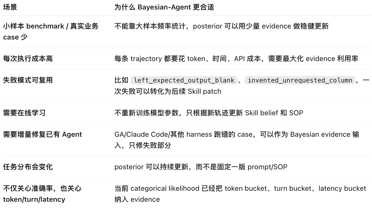
总结
三门问题告诉我们:信息不是“看起来还剩几个选项”,而是“这个证据在不同假设下出现的概率是多少”。
Bayesian Evidence Model 告诉我们:当证据由多个特征组成时,可以用一个可解释的 likelihood model,把每个特征对成功或失败的贡献统计出来;目前采用的是 factorized categorical likelihood,后续可以替换成更强的贝叶斯模型。
人的后天学习告诉我们:技能不是一次性写死的规则,而是在经验、反馈和训练中不断校准的操作假设。
Bayesian-Agent 把这些思想落到 LLM Agent 工程里:
Skill = hypothesis
Trajectory = evidence
Verifier = supervision
Evidence Model = posterior update
Context = non-parametric learned state
Next run = acquired learning in action
这就是为什么我们认为 Skill/SOP 的进化会成为 Agent 工程里的核心能力。大模型已经足够聪明,但真正可靠的 Agent 还需要学会一件更基础也更困难的事:从自己的成功经验和失败教训中,持续后天学习。